Riemann Integral

This article/section deals with mathematical concepts appropriate for late high school or early college.

The Riemann integral is the mathematical definition of the integral of a function, that is, a measure of the area enclosed by its graph in calculus. The term, along with Riemann sum, is also a useful method for approximating that area.

How the Riemann integral works. The blue region shows the lower estimate of the strip areas, blue+yellow is the actual function area, and blue+yellow+pink is the upper estimate. Yellow+pink is the difference between the low and high estimates.

Theoretical Introduction

The Riemann integral is the correct term for the theoretical definition, given by Bernhard Riemann around 1853, for the integral of a function.

The integral of a function is generally conceptualized as measuring the area under the graph of that function.

Specifically, the area between two specific points, and , is called the definite integral, written

The "obvious" way to evaluate such an integral is to divide the domain of the function into many small intervals (this division is called a mesh) and to visualize the area under the function as being the sum of the areas of the rectangular strips created by the mesh. The height of each strip is hard to measure accurately, because the function value is typically not constant across the interval. What is done is to choose some value that approximately represents the function value on the interval, multiply by the interval width (strip width) and take that as the area of the strip. The representation of the function value is generally taken as

• The function value at the left edge of the interval.
• The function value at the right edge of the interval.
• The function value at the center of the interval.
• The maximum function value across the interval.
• The minimum function value across the interval.
• Some other trick, such as the use of Simpson's rule; see below.

The use of the minimum and maximum values are particularly interesting, both practically and theoretically. If the minimum value is used, one knows that the resultant sum of the strip areas must be less than or equal to the true area. Conversely, the maximum value will give a resultant sum greater than or equal to the true area. Hence one can make guarantees of accuracy—if the strip widths are narrow enough that the two values obtained are within one millionth of each other, one knows that this is within one millionth of the true result.

The breaking down of the function graph into rectangular strips, and approximating the area under the graph in terms of rectangles, is a very well-known technique, and is what is commonly called the "Riemann integral", or, more properly, the "Riemann sum". Most of the rest of this article is about it. However, Bernhard Riemann's contribution to this, and the reason we name it after him, is his theoretical achievement. (Reimann was a brilliant theoretical mathematician. He essentially invented the field of differential geometry, as well as making major contributions to number theory and other areas.)

What Riemann did was to show that, if one takes the minimum and maximum values (as described above), and makes the strips narrower and narrower, (the mesh finer and finer), the two approximations will converge to each other. That is, they will approach the same value as a limit. Mathematicians take that limit as the definition of the (Riemann) integral. So Riemann's achievement was to take the common computational task of adding up the strip areas, and make a proper (or, as mathematicians say, rigorous) definition out of it. In so doing, he put the definite integral, and hence integral calculus, on a firm theoretical basis.

Riemann's proof is beyond the scope of this article. It applies to any function which is either continuous or has a finite number of discontinuities. (At a more advanced level, it applies to any function for which the set of discontinuities has measure zero.)

To define the limit, he had to modify the usual "epsilon/delta" formulation. The definition is this (see the "limit" article):

For every epsilon greater than zero, there is a mesh such that, for that mesh and all finer meshes (put in additional subdivision points), the difference between the upper sum (using the maximum function value) and the lower sum (using the minimum value) is less than epsilon.

Introduction to the Applied Method

As a geometric interpretation of the area under a curve (also called the definite integral), the Riemann integral consists of dividing the area under the curve of the function into fixed width subintervals. The area of each subinterval is added together to get the approximation. The greater the number of subintervals that is used, the closer the approximation is to the true value of the integral, where the "true value" is defined as that value obtained in the limit as the width of the subintervals approaches zero. Only if the limit exists does the integral exist.

Most of the time, rectangles are used when evaluating the area. Sometimes more complex shapes, such as parabolas in Simpson's rule, are used in approximations.

Evaluating a Riemann Integral

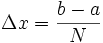
The domain of the function is partitioned into segments. These segments are called subintervals of the partition. If each subinterval is of equal width, then width can be represented by

.

To find the area under the curve, the areas of all subintervals are added together. With each shape of subintervals, there are different equations used to evaluate the area. If the subintervals are rectangles, we can use the properties of rectangles to find the area. The area of a rectangle is height times width. To get the height of the rectangles, we evaluate the function at the subinterval.

The equation for the area of each rectangle is

.

For simplification, we can say that

.

There are three methods of evaluating the area of each rectangle. The function could be evaluated at the left, right, or midpoint of each subinterval.

The three equations are as follows:

Left Endpoint:

Right Endpoint:

Midpoint:

If we increase the number of partitions, N the summation is a closer approximation of the true area under the curve. This can be written as

Example

Part A

How evaluating a Riemann Integral works.
Given:

To begin, let's set:

This means:

For this example, we'll go with the Left Endpoint approximation. This gives us:

For an approximation, this result is horrible. The actual value is 1/3. To increase our accuracy, we must increase the number of subintervals, . This time:

This result is closer, but nowhere near as accurate as we want it to be.

As we increase , our approximation approaches the real value. To find the real value, we must use the limit function.

Part B

To get the exact value of the integral, we must find:

We know that:

So we can say:

Because is not dependent on , we can separate this into two summations and solve them separately.
The first part:

We know from the sequence of Square pyramidal numbers that:

This says that the sum of consecutive integers is equal to:

We can apply that to our problem, to get:

We can now simplify the second part.

This gives us:

We can now simplify this using L'Hôpital's Rule

is gone from the limit, and we are left with a constant.

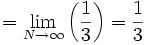
Therefore:

Part C

Say that, instead of evaluating the integral from 0 to 1, we wanted to solve it from 0 to an undetermined upper limit, c:

This changes our value:

This actually does not change any calculations until we replace in the limit.

Because is a constant, we can factor it out of the limit.

We know from above how to simplify what is in the limit, so we are left with:

Therefore:

We can rewrite this as:

Where is known as the constant of integration which is necessary here since we have performed an indefinite integration - that is integrated without specifying the limits of integration. This is done because any constant will give you a function that has the desired derivative.

See also

• Integral
• Bernhard Riemann
• Simpson's rule