Calc3.1

Introduction and Prerequisites

Welcome to Multivariate Calculus! This course will move quickly, and cover a lot of ground. For this reason, the instructors personal email and phone number will be available to students. We will begin with a discussion of functions of multiple variables, including differentiaion and integration, and move on to more complicated matters associated with these functions, such as optimization with constraints, surface integrals, and the basics of differential geometry. It will cover the same material as a University-level Calculus 3 course, but we will begin with a review of concepts from Calculus 2 that the student should already be familiar with.

It is essential that the student have firm grasp of concepts from Calculus 1. This includes, but is not limited to,

• Limits of functions of a single variable, including L'Hopitals rule,
• Differention of a function of a single variable,
• Integration of a function of a single variable, including integration by parts,
• The fundamental theorem of calculus
• Analytic geometry of the plane, including arc length calculations
• Infinite series, including the classic convergence tests and methods of calculation

Course Outline

Lecture 1

• Introduction and Course Outline

• Review: Single variable calculus

• Geometry in Three Dimensions

• Scalar Functions in Two and Three Dimensions

Lecture 2

• Vectors, and Vector Functions

• Coordinate Systems

• Limits of Multiariate Functions

• Elementary Vector Calculus

• Partial Derivatives

Lecture 3

• Directional Derivatives

• The Gradient

• Parametric Curves and Surfaces

• Extrema of Multivariate Functions

• Optimization with Constraints: Langrage Multipliers

Lecture 4

• The Tangent Plane

• The Frenet Frame

• Curvature of a Curve

Lecture 5

• The Double Integral

• Double Integrals in Different Coordinate Systems

• Double Integral Applications

Lecture 6

• The Triple Integral

• Triple Integrals in Different Coordinate Systems

• Triple Integral Applications

Lecture 7

• Review:Vector Functions

• Review:Matrix Algebra

• The Divergence

• The Curl

• Applications of the Divergence and Curl

Lecture 8

• Generalized Integration

• The Line Integral

• Green's Theorem in the Plane

• The Surface Integral

Lecture 9

• Greens Theorem

• Gauss' Theorem

• Stokes Theorem

• Applications

Lecture 10

• The Exterior Derivative

• Applications: The Maxwell Equations

• Generalized Stokes Theorem

Lecture 11

• Review:Ordinary Differential Equations

• Linear Partial Differential Equations

• The Cauchy-Riemann Operator

Lecture 12

• The Wave Equation

Lecture 13

• The Heat Equation

Lecture 14

• Course Review

Single Variable Review

This section is not intended to be a course in elementary calculus - the student is expected to understand this material before beginning the course. It is provided here as a reference for student.

We begin with a review of functions. Functions, in the most general sense, are rules which associate one thing with another. For example, there is a function which takes a place on Earth and returns its temperature - in that case, the "domain" of the function is the Earth, and the "range" are temperatures. In elementary calculus, the domain and the range tend to be subsets of the real numbers. In this course, the domain and range may be real numbers, or sets of vectors in higher dimensions, or matrix sets.

The limit of a function is defined so that if, for any , there is an such that every number within of is taken by the function to a number within of .

The derivative of a function is the limit and is the slope of the line tangent to the function's curve at . To write the derivative of a function with respect to , we write or .

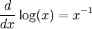
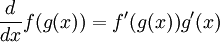
Some special derivative bear reviewing:

The indefinite integral or antiderivative of a function is any function such that .

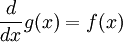The definite integral, or as it is defined in elementary calculus, the Riemann sum, is a quantity EXPAND THIS

The fundamental theorem of calculus states that .

The material just described should be so familiar to the student that it can be recited as easily as multiplication tables or trigonometric values on the unit circle.

Geometry in Three Dimensions

In three dimensions, we most often work with the xyz coordinate system. This system is called "right handed," because if we take our right palm, with our knuckles pointing in the positive x direction, and bend our fingers so that they point in the positive y direction, our thumbs automatically point in the positive z direction. See illustration.

We are familiar with the basic geometry of the plane already, but a brief review will help illustrate the concepts we encounter in the next dimension.

Any line in the xy plane can be described as , where is the "slope" and is the y-intercept. When we raise the number of dimensions, we see how similar the equation of a plane is in three-space: 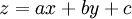, where is the slope along the x-axis, etc. See illustration.

Describing a line in three dimensions is trickier, and requires what is called a parametric equation. This method of describing lines relies on some variable which isn't a coordinate, like time, to describe a point as it travels through space. For example, if a point is at some location at time , and then over 1 second travels feet in the x direction, feet in the y direction, and feet in the z direction, we can descrive its location at any time as . As it travels, this point traces out a line.

Scalar Functions

Scalar functions are the kinds of functions you're used to, but in more dimensions. The example given earlier of a