Quantitative Introduction to General Relativity

For a general overview of the theory, see General Relativity

This article/section deals with mathematical concepts appropriate for a student in late university or graduate level.

General Relativity is a mathematical extension of Special Relativity. GR views space-time as a 4-dimensional manifold, which looks locally like Minkowski space, and which acquires curvature due to the presence of massive bodies. Thus, near massive bodies, the geometry of space-time differs to a large degree from Euclidean geometry: for example, the sum of the angles in a triangle is not exactly 180 degrees. Just as in classical physics, objects travel along geodesics in the absence of external forces. Importantly though, near a massive body, geodesics are no longer straight lines. It is this phenomenon of objects traveling along geodesics in a curved spacetime that accounts for gravity.

The mathematical expression of the theory of general relativity takes the form of the Einstein field equations, a set of ten nonlinear partial differential equations. While solving these equations is quite difficult, examining them provides valuable insight into the structure and meaning of the theory.

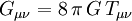
In their general form, the Einstein field equations are written as a single tensor equation in abstract index notation relating the curvature of spacetime to sources of curvature such as energy density and momentum.

In this form, represents the Einstein tensor, is the same gravitational constant that appears in the law of universal gravitation, and is the stress-energy tensor (sometimes referred to as the energy-momentum tensor). The indices and range from zero to three, representing the time coordinate and the three space coordinates in a manner consistent with special relativity. is the cosmological constant.

The left side of the equation — the Einstein tensor — describes the curvature of spacetime in the region under examination. The right side of the equation describes everything in that region that affects the curvature of spacetime.

As we can clearly see even in this simplified form, the Einstein field equations can be solved "in either direction." Given a description of the gravitating matter, energy, momentum and fields in a region of spacetime, we can calculate the curvature of spacetime surrounding that region. On the other hand, given a description of the curvature of a region spacetime, we can calculate the motion of a test particle anywhere within that region.

Even at this level of examination, the fundamental thesis of the general theory of relativity is obvious: motion is determined by the curvature of spacetime, and the curvature of spacetime is determined by the matter, energy, momentum and fields within it.

The right side of the equation: the stress-energy tensor

In the Newtonian approximation, the gravitational vector field is directly proportional to mass. In general relativity, mass is just one of several sources of spacetime curvature. The stress-energy tensor, , includes all of these sources. Put simply, the stress-energy tensor quantifies all the stuff that contributes to spacetime curvature, and thus to the gravitational field.

First we will define the stress-energy tensor technically, then we'll examine what that definition means. In technical terms, the stress energy tensor represents the flux of the component of 4-momentum across a surface of constant coordinate .

Fine. But what does that mean?

In classical mechanics, it's customary to refer to coordinates in space as , and . In general relativity, the convention is to talk instead about coordinates , , , and , where is the time coordinate otherwise called , and the other three are just the , and coordinates. So "a surface of constant coordinate "" simply means a 3-plane perpendicular to the axis.

The flux of a quantity can be visualized as the magnitude of the current in a river: the flux of water is the amount of water that passes through a cross-section of the river in a given interval of time. So more generally, the flux of a quantity across a surface is the amount of that quantity that passes through that surface.

Four-momentum is the special relativity analogue of the familiar momentum from classical mechanics, with the property that the time coordinate of a particle's four-momentum is simply the energy of the particle; the other three components of four-momentum are the same as in classical momentum.

So putting that all together, the stress-energy tensor is the flux of 4-momentum across a surface of constant coordinate. In other words, the stress-energy tensor describes the density of energy and momentum, and the flux of energy and momentum in a region. Since under the mass-energy equivalence principle we can convert mass units to energy units and vice-versa, this means that the stress-energy tensor describes all the mass and energy in a given region of spacetime.

Put even more simply, the stress-energy tensor represents everything that gravitates.

The stress-energy tensor, being a tensor of rank two in four-dimensional spacetime, has sixteen components that can be written as a 4 × 4 matrix.

Here the components have been color-coded to help clarify their physical interpretations.

energy density, which is equivalent to mass-energy density; this component includes the mass contribution

, ,

the components of momentum density

, ,

the components of energy flux

The space-space components of the stress-energy tensor are simply the stress tensor from classic mechanics. Those components can be interpreted as:

, , , , ,

the components of shear stress, or stress applied tangential to the region

, ,

the components of normal stress, or stress applied perpendicular to the region; normal stress is another term for pressure.

Pay particular attention to the first column of the above matrix: the components , , and , are interpreted as densities. A density is what you get when you measure the flux of 4-momentum across a 3-surface of constant time. Put another way, the instantaneous value of 4-momentum flux is density.

Similarly, the diagonal space components of the stress-energy tensor — , and — represent normal stress, or pressure. Not some weird, relativistic pressure, but plain old ordinary pressure, like what keeps a balloon inflated. Pressure also contributes to gravitation, which raises a very interesting observation.

Imagine a box of air, a rigid box that won't flex. Let's say that the pressure of the air inside the box is the same as the pressure of the air outside the box. If we heat the box — assuming of course that the box is airtight — then the temperature of the gas inside will rise. In turn, as predicted by the ideal gas law, the pressure within the box will increase.

The box is now heavier than it was.

More precisely, increasing the pressure inside the box raised the value of the pressure contribution to the stress-energy tensor, which will increase the curvature of spacetime around the box. What's more, merely increasing the temperature alone caused spacetime around the box to curve more, because the kinetic energy of the gas molecules inside the box also contributes to the stress-energy tensor, via the time-time component . All of these things contribute to the curvature of spacetime around the box, and thus to the gravitational field created by the box.

Of course, in practice, the contributions of increased pressure and kinetic energy would be miniscule compared to the mass contribution, so it would be extremely difficult to measure the gravitational effect of heating the box. But on larger scales, such as the sun, pressure and temperature contribute significantly to the gravitational field.

In this way, we can see that the stress-energy tensor neatly quantifies all static and dynamic properties of a region of spacetime, from mass to momentum to electric charge to temperature to pressure to shear stress. Thus, the stress-energy tensor is all we need on the right-hand side of the equation in order to relate matter, energy and, well, stuff to curvature, and thus to the gravitational field.

Example 1: Stress-energy tensor for a vacuum

The simplest possible stress-energy tensor is, of course, one in which all the values are zero.

This tensor represents a region of space in which there is no matter, energy or fields, not just at a given instant, but over the entire period of time in which we're interested in the region. Nothing exists in this region, and nothing happens in this region.

So one might assume that in a region where the stress-energy tensor is zero, the gravitational field must also necessarily be zero. There's nothing there to gravitate, so it follows naturally that there can be no gravitation.

In fact, it's not that simple. We'll discuss this in greater detail in the next section, but even a cursory qualitative examination can tell us there's more going on than that. Consider the gravitational field of an isolated body. A test particle placed somewhere near but outside of the body will move in a geodesic in spacetime, freely falling inward toward the central mass. A test particle with some constant linear velocity component perpendicular to the interval between the particle and the mass will move in a conic section. This is true even though the stress-energy tensor in that region is exactly zero. This much is obvious from our intuitive understanding of gravity: gravity affects things at a distance. But exactly how and why this happens, in the model of the Einstein field equations, is an interesting question which will be explored in the next section.

Example 2: Stress-energy tensor for an ideal dust

Imagine a time-dependent distribution of identical, massive, non-interacting, electrically neutral particles. In general relativity, such a distribution is called a dust. Let's break down what this means.

time-dependent

The distribution of particles in our dust is not a constant; that is to say, the particles may be motion. The overall configuration you see when you look at the dust depends on the time at which you look at it, so the dust is said to be time-dependent.

identical

The particles that make up our dust are all exactly the same; they don't differ from each other in any way.

massive

Each particle in our dust has some rest mass. Because the particles are all identical, their rest masses must also be identical. We'll call the rest mass of an individual particle .

non-interacting

The particles don't interact with each other in any way: they don't collide, and they don't attract or repel each other. This is, of course, an idealization; since the particles are said to have mass , they must at least interact with each other gravitationally, if not in other ways. But we're constructing our model in such a way that gravitational effects between the individual particles are so small as to be be negligible. Either the individual particles are very tiny, or the average distance between them is very large. This same assumption neatly cancels out any other possible interactions, as long as we assume that the particles are far enough apart.

electrically neutral

In addition to the obvious electrostatic effect of two charged particles either attracting or repelling each other — thus violating our "non-interacting" assumption — allowing the particles to be both charged and in motion would introduce electrodynamic effects that would have to be factored into the stress-energy tensor. We would greatly prefer to ignore these effects for the sake of simplicity, so by definition, the particles in our dust are all electrically neutral.

The easiest way to visualize an ideal dust is to imagine, well, dust. Dust particles sometimes catch the light of the sun and can be seen if you look closely enough. Each particle is moving in apparent ignorance of the rest, its velocity at any given moment dependent only on the motion of the air around it. If we take away the air, each particle of dust will continue moving in a straight line at a constant velocity, whatever its velocity happened to be at the time. This is a good visualization of an ideal dust.

We're now going to zoom out slightly from our model, such that we lose sight of the individual particles that make up our dust and can consider instead the dust as a whole. We can fully describe our dust at any event — where event is defined as a point in space at an instant in time — by measuring the density and the 4-velocity at . If we have those two pieces of information about the dust at every point within it at every moment in time, then there's literally nothing else to say about the dust: it's been fully described.

Density

Let's start by figuring out the density of dust at a the event , as measured from the perspective of an observer moving along with the flow of dust at . The density is calculated very simply:

where is the mass of each particle and is the number of particles in a cubical volume one unit of length on a side centered on . This quantity is called proper density, meaning the density of the dust as measured within the dust's own reference frame. In other words, if we could somehow imagine the dust to measure its own density, the proper density is the number it would get.

Clearly proper density is a function of position, since it varies from point to point within the dust; the dust might be more "crowded" over here, less "crowded" over there. But it's also a function of time, because the configuration of the dust itself is time-dependent. If you measure the proper density at some point in space at one instant of time, then measure it at the same point in space at a different instant of time, you may get a different measurement. By convention, when dealing with a quantity that depends both on position in space and on time, physicists simply say that the quantity is a function of position, with the understanding that they're referring to a "position" in four-dimensional spacetime.

4-velocity

The other quantity we need is 4-velocity. Four-velocity is an extension of three-dimensional velocity (or 3-velocity). In three dimensional space, 3-velocity is a vector with three components. Likewise, in four-dimensional spacetime, 4-velocity is a vector with four components.

Directly measuring 4-velocity is an inherently tricky business, since one of its components describes motion along a "direction" that we cannot see with our eyes: motion through time. The math of special relativity lets us calculate the 4-velocity of a moving particle given only its 3-velocity (with components where ) and the speed of light. The time component of 4-velocity is given by:

and the space components , and by:

where is the boost, or Lorentz factor:

and where , in turn, is the square of the Euclidean magnitude of the 3-velocity vector :

Therefore, if we know the 3-velocity of the dust at event , then we can calculate its 4-velocity. (For more details on the how and why of 4-velocity, refer to the article on special relativity.)

Just as proper density is a function of position in spacetime, 4-velocity also depends on position. The 4-velocity of our dust at a given point in space won't necessarily be the same as the 4-velocity of the dust at another point in space. Likewise, the 4-velocity at a given point at a given time may not be the same as the 4-velocity of the dust at the same point at a different time. It helps to think of 4-velocity as the velocity of the dust through a point in both space and time.

Assembling the stress-energy tensor

Since the density and the 4-velocity fully describe our dust, we have everything we need to calculate the stress-energy tensor.

where the symbol indicates a tensor product. The tensor product of two vectors is a tensor of rank two, so the stress-energy tensor must be a tensor of rank two. In an arbitrary coordinate frame , the contravariant components of the stress-energy tensor for an ideal dust are given by:

From this equation, we can now calculate the contravariant components of the stress-energy tensor for an ideal dust.

Time-time component

We start with the contravariant time-time component :

If we rearrange the terms in this equation slightly, something important becomes apparent:

Recall that is a density quantity, in mass per unit volume. By the mass-energy equivalence principle, we know that . So we can interpret this component of the stress-energy tensor, which is written here in terms of mass-energy, to be equivalent to an energy density.

Off-diagonal components

The off-diagonal components of the tensor — where and are not equal — are calculated this way:

Again, recall that is a quantity of mass per unit volume. Multiplying a mass times a velocity gives momentum, so we can interpret as the density of momentum along the direction, multiplied by constants and . Momentum density is an extremely difficult quantity to visualize, but it's a quantity that comes up over and over in general relativity. If nothing else, one can take comfort in the fact that momentum density is mathematically equivalent to the product of mass density and velocity, both of which are much more intuitive quantities.

Note that the off-diagonal components of the tensor are equal to each other:

In other words, in the case of an ideal dust, the stress-energy tensor is said to be symmetric. A rank two symmetric tensor is said to be symmetric if .

Diagonal space components

The diagonal space components of the stress-energy tensor are calculated this way:

In this case, we're multiplying a four-dimensional mass density, , by the square of a component of 4-velocity. By dimensional analysis, we can see:

Recall that the force has units:

If we divide the units of the diagonal space component by the units of force, we get:

So the diagonal space components of the stress-energy tensor come are expressed in terms of force per unit volume. Force per unit area are, of course, the traditional units of pressure in three-dimensional mechanics. So we can interpret the diagonal space components of the stress-energy tensor as the components of "4-pressure" in spacetime.

The big picture

We now know everything we know to assemble the entire stress-energy tensor, all sixteen components, and look at it as a whole.

The large-scale structure of the tensor now becomes apparent. This is the stress-energy tensor of an ideal dust. The tensor is composed entirely out of the proper density and the components of 4-velocity. When velocities are low, the coefficient , even though it's a squared value, remains extremely close to one.

The time-time component includes a mass multiplied by the square of the speed of light, so it has to do with energy. The rest of the top row and left column all include the speed of light as a coefficient, as well as density and velocity; in the case of an ideal dust which is made up of non-interacting particles, the energy flux along any basis direction is the same as the momentum density along that direction. This is not the case in other, less simple models, but it's true here.

The diagonal space components of the tensor represent pressure. For example, the component represents the pressure that would be exerted on a plane perpendicular to the direction.

The off-diagonal space components represent shear stress. The component, for instance, represents the pressure that would be exerted in the direction on a plane perpendicular to the axis.

The overall process for calculating the stress-energy tensor for any system is fairly similar to the example given here. It involves taking into account all the matter and energy in the system, describing how the system evolves over time, and breaking that evolution down into components which represent individual densities and fluxes along different directions relative to a chosen coordinate basis.

As can easily be imagined, the task of constructing a stress-energy tensor for a system of arbitrary complexity can be a very daunting one. Fortunately, gravity is an extremely weak interaction, as interactions go, so on the scales where gravity is interesting, much of the complexity of a system can be approximated. For instance, there is absolutely nothing in the entire universe that behaves exactly like the ideal dust described here; every massive particle interacts, in one way or another, with other massive particles. No matter what, a real system is going to be very much more complex than this approximation. Yet, the ideal dust solution remains a much-used approximation in theoretical physics specifically because gravity is such a weak interaction. On the scales where gravity is worth studying, many distributions of matter, including interstellar nebulae, clusters of galaxies, even the whole universe really do behave very much like an ideal dust.

The left side of the equation: the Einstein curvature tensor

We will recall that the Einstein field equations can be written as a single tensor equation:

The right side of the equation consists of some constants and the stress-energy tensor, described in significant detail in the previous section. The right side of the equation is the "matter" side. All matter and energy in a region of space is described by the right side of the equation.

The left side of the equation, then, is the "space" side. Matter tells space how to curve, and space tells matter how to move. So the left side of the Einstein field equation must necessarily describe the curvature of spacetime in the presence of matter and energy.

Some assumptions about the universe

Before we proceed into a discussion of what curvature is and how the Einstein equation describes it, we must first pause to state some fundamental assumptions about the universe.

The first assumption we're going to make is that spacetime is continuous. In essence, this means that for any event in spacetime — that is, any point in space and moment in time — there exists some local neighborhood of where the intrinsic properties of spacetime differ from those at by only an infinitesimal amount.

The second assumption we're going to make is that spacetime is differentiable everywhere. In other words, the geometry of spacetime doesn't have any sharp creases in it.

If we hold these two assumptions to be true, then a convenient property of spacetime emerges: Given any event , there exists a local neighborhood where spacetime can be treated as flat, that is, having zero curvature. It is not necessarily true that all of spacetime be flat — in fact, it most definitely is not — but given any event in spacetime, there exists some neighborhood around it that is flat. This neighborhood may be arbitrarily small in both time and space, but it is guaranteed to exist as long as our two assumptions remain valid.

With these two assumptions and this convenient property in hand, we will now examine what it means to say that spacetime is curved.

Flatness versus curvature

Let's start by considering the simplest possible geometry: the Euclidean plane.

The Euclidean plane is an infinite, flat, two-dimensional surface. A sheet of paper is a good approximation of the Euclidean plane. Onto this plane, we can project a set of Cartesian coordinates. By "Cartesian," we mean that the coordinate axes are straight lines, that they are perpendicular, and that the unit lengths of the axes are equal. A fancier term for a Cartesian coordinate system is an orthonormal basis.

Note carefully the distinction between the Euclidean plane and Cartesian coordinates. The plane exists as a thing in and of itself, just as a blank piece of paper does. It has certain properties, which we'll get into below. Those properties are intrinsic to the plane. That is, the properties don't have anything to do with the coordinates we project onto the plane. The plane is a geometric object, and the coordinates are the method by which we measure the plane. (The emphasis on the word measure there is not accidental; please keep this idea in the foreground of your mind as we continue.)

Cartesian coordinates are not the only coordinates we can use in the Euclidean plane. For example, instead of having axes that are perpendicular to each other, we could choose axes that are straight lines, but that meet at some non-perpendicular angle. These types of coordinates are called oblique.

For that matter, we're not bound to use straight-line coordinates at all. We could instead choose polar coordinates, wherein every point on the plane is described by a distance from a fixed but arbitrary point and an angle from a fixed but arbitrary direction. Polar coordinates are often more convenient than Cartesian coordinates. For example, when navigating a ship on the ocean, the location of a fixed point is usually described in terms of a bearing and a distance, where the distance is the straight-line distance from the ship to the point, and the bearing is the clockwise angle relative to the direction in which the ship is sailing. Polar coordinates in two and three dimensions are often used in physics for similar reasons.

But there's a fundamental problem with polar coordinates that is not present with Cartesian coordinates. In Cartesian coordinates, every point on the Euclidean plane is identified by exactly one set of real numbers: there is precisely one set of and coordinates for every point, and every point corresponds to precisely one set of coordinates.

This is not true in polar coordinates. What are the unique polar coordinates for the origin? The radial distance is obviously zero, but what is the angle? In actuality, if the radial distance is zero, any angle can be used, and the coordinates will identify the same point. The one-to-one correspondence between points in the plane and pairs of coordinates breaks down at the origin.

In mathematical terms, polar coordinates in the Euclidean plane have a coordinate singularity at the origin. A coordinate singularity is a point in space where ambiguities are introduced, not because of some intrinsic property of space, but because of the coordinate basis you chose.

So clearly there may exist a reason to choose one coordinate system over another when measuring — there's that word again — the Euclidean plane. Polar coordinates have a singularity at the origin — in this case, a point of undefined angle — while Cartesian coordinates have no such singularities anywhere. So there may be good reason to choose Cartesian coordinates over polar coordinates when measuring the Euclidean plane.

Fortunately, this is always possible. The Euclidean plane can always be measured by Cartesian coordinates; that is, coordinates wherein the axes are straight and perpendicular at their intersection, and where lines of constant coordinate — picture the grid on a sheet of graph paper — are always a constant distance apart no matter where you measure them.

Imagine taking a piece of graph paper, which is printed in a pattern that lets us easily visualize the Cartesian coordinate system, and rolling it into a cylinder. Do any creases appear in the paper? No, it remains smooth all over. Do the lines printed on the paper remain a constant distance apart everywhere? Yes, they do. In technical mathematical terms, then, the surface of a cylinder is flat. That is, it can be measured by an orthonormal basis, and there is everywhere a one-to-one correspondence between sets of coordinates and points on the surface. It's possible not to use an orthonormal basis to measure the surface; one might reasonably choose polar coordinates, or some other arbitrary coordinate system, if it's more convenient. But whichever basis is actually used, it's always possible to switch to an orthonormal basis instead.

Now imagine wrapping a sheet of graph paper around a basketball. Does the paper remain smooth? No, if we press it down, creases appear. Do the lines on the paper remain parallel? No, they have to bend in order to conform the paper to the shape of the ball. In the same technical mathematical terms, the surface of a sphere is not flat. It's curved. That is, it is not possible to measure the surface all over using an orthonormal basis.

But what if we focus our attention only on a part of the sphere? What if instead of measuring a basketball, we want to measure the whole Earth? The Earth is a sphere, and therefore its surface is curved and can't be measured all over with Cartesian coordinates. But if we look only at a small section of the surface — a square mile on a side, for instance — then we can project a set of Cartesian coordinates that work just fine. If we choose our region of interest to be sufficiently small, then Cartesian coordinates will fit on the surface to within the limits of our ability to measure the difference.

The surface of a sphere, then, is globally curved, but locally flat. In physicist jargon, the surface of a sphere can be flattened over a sufficiently small region. Not the whole sphere all at once, nor half of it, nor a quarter of it. But a sufficiently small region can be dealt with as if it were a Euclidean plane.

But this brings up an important point. The entire surface of the sphere is curved, and thus can't be approximated with Cartesian coordinates. But a sufficiently small patch of the surface can be approximated with Cartesian coordinates. This implies, then, that "curvedness" isn't an either-or property. Somewhere between the locally flat region of the surface and the entire surface, the amount of curvature goes from none to some value. Curvature, then, must be something we can measure.

The metric tensor

It is a fundamental property of the Euclidean plane that, when Cartesian coordinates are used, the distance between any two points and is given by the following equation:

where and are the distance between and in the and directions, respectively. This is essentially a restatement of the universally known Pythagorean theorem, and in the context of general relativity, it is called the metric equation. Metric, of course, comes from the same linguistic root as the word measure, and since this is the equation we use to measure distances, it makes sense to call it the metric equation.

But this particular metric equation only works on the Euclidean plane with Cartesian coordinates. If we use polar coordinates, this equation won't work. If we're on a curved surface instead of a plane, this equation won't work. This metric equation is only valid on a flat surface with Cartesian coordinates.

Which makes it pretty useless, since so much of physics revolves around curved spacetime and spherical coordinates.

What we need is a generalized metric equation, some way of measuring the interval of any two points regardless of what coordinate system we're using or whether our local geometry is flat or curved.

The metric tensor equation provides this generalization.

If is any vector having components , the length of is given by the following equation:

where is the metric tensor, and and range over the number of dimensions. Recall that Einstein summation notation means that this is actually a sum over indices and . If we assume that we're in the two-dimensional Euclidean plane, the metric tensor equation expands to:

The terms of the metric tensor, then, must be numerical coefficients in the metric equation. We already know what these equations need to be to make the metric equation work in the Euclidean plane with Cartesian coordinates:

Now we can write the metric tensor for the Euclidean plane in Cartesian coordinates in the form of a 2 × 2 matrix:

So in the case of the Euclidean plane with Cartesian coordinates, the metric tensor is the Kronecker delta:

Of course, the same concepts apply if we expand our interest from the plane to three-dimensional Euclidean space with Cartesian coordinates. We just have to let the indices of the Kronecker delta run from 1 to 3.

Which gives us the following metric equation for the length of a vector (omitting terms with zero coefficient):

Which precisely agrees with the Pythagorean theorem in three dimensions. So given a metric tensor for any space and coordinate basis, we can calculate the distance between any two points. The metric tensor, therefore, is what allows us to measure curved space. In a very real sense, the metric tensor describes the shape of both the underlying geometry and the chosen coordinate basis.

But relativity is concerned not with geometrically abstract space; we're interested in very real spacetime, and that requires a slightly different kind of metric.